Modelling Rabbit Populations; an Introduction to Chaos Theory
Non-linear systems; those systems that can't be solved analytically (read, nicely) are essentially what I spent the whole last year of my maths degree specialising in. They are equations that attempt to model things which lead to chaos, such as weather systems, the flow of fluids and populations. By chaos I mean that if we slightly changed the initial conditions, then a short time down the line we have a completely different situation: the butterfly effect. I'm writing this article with A Level Maths students in mind as an introduction to chaos theory, so I'm going to sanitise the maths and present one of the common problems that people first meet when they study this topic.
We are going to be modelling the population of a colony of rabbits living on an island. We are going to have Xn represent the proportion of rabbits that there are out of the maximum possible number of rabbits that there are on an island. So if Xn=1 that means the island is completely full of rabbits and if Xn=0 that means the island is completely empty.
Rabbits are famously quite into breeding, so if you have lots of rabbits which are able to breed, you will get more the next year and so the number of rabbits the next year would go up proportional to the number of rabbits that there were in the year before which was Xn. However, there is only so much food available on the island and so if there are too many rabbits on the island then there won't be enough food. We model this part by adding that the population should also be proportional the food availability which is (1-Xn). Thus the number of rabbits in the next year Xn+1 would be proportional to Xn(1-Xn). We are going to write this as the iterative equation Xn+1=kXn(1-Xn) where k is the constant of proportionality.
We can vary the value of k to be whatever we like and you can think of it as representing the virility of the rabbits. If it is 0 then the rabbits are rubbish at breeding and die off immediately. Let's look at what happens with some larger values of k. Each time we will start the warren off at half capacity, so the initial population will be 0.5:
There's lots to analyse here; we'll start from the left. When k=0.5 the rabbits didn't fair much better than when k=0. Every generation the rabbits are failing to replace themselves and so there are even fewer potential parents. This leads to colony collapse very quickly. Any value of k<1 leads to this behaviour.
As we increase k to 1.8 and 2.4 we see that the population stabilises by tending towards some constant number. This is ideally what the rabbits are after and if any event temporally changed the number of rabbits for a generation their population would bounce back to these constant states. This stability occurs between 1<k<3.
As we go above that k=3 threshold we get more complicated patterns arise as shown by k=3.3 and k=3.5. These rabbits are such successful breeders that even with a small number of parents they are able to produce loads of offspring. Unfortunately these children are simply too many for the island to support and so come the next season we end up with most dying out and so the population returns to a lower level. k=3.3 is jumping between two states, but k=3.5 is exhibiting a more complex pattern of jumping between a low, a medium and a high state. We'll come back to explore what is happening for these later on, but for all values of k<4 the pattern becomes more and more chaotic with the population jumping all over the place (hop hop).
Finally the whole pattern gets simpler again for 4<k. In the k=4.5 case we immediately get the population rise to way above the carrying capacity of the island. They eat every food source and go extinct by the next year. The case just gets worse and worse as you increase k. Clearly the negative numbers of rabbits in the table, so we must assume that they just drop to zero.
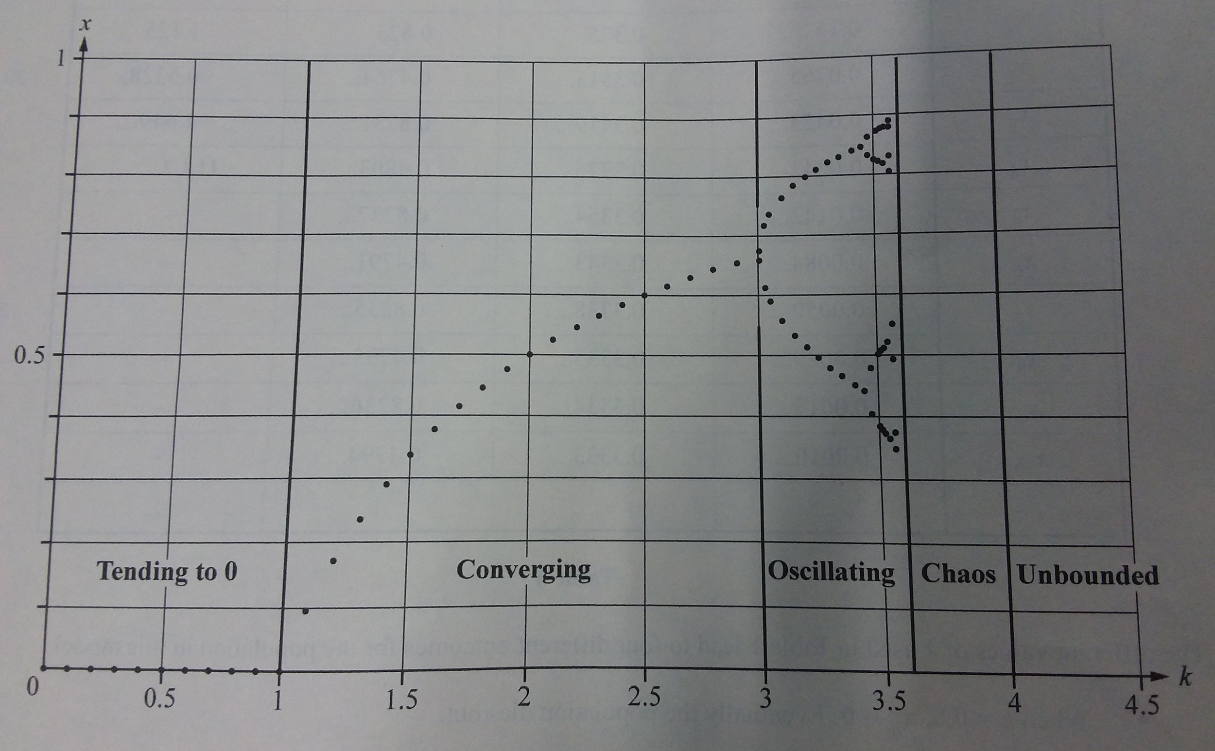
In short, we have five cases. Dying from infertility, stable populations, oscillating populations, chaos or dying from overpopulation.
A graph showing the different regions. The Chaos region would be fractally.
As you can see, the first split into having two states happens at k=3, but after a shorter and shorter increase of k we get more and more doublings of stable states. By the time it gets anywhere close to k=4 it has been split so many times that even a small change in the value of k (or the number of starting rabbits) leads to dramatically different behaviour. This is the definition of chaos. The splitting of these stable states is called bifurcation and they come up again and again in chaos theory.
In 1975 a mathematician named Mitchell Feigenbaum was investigating this model of populations and he notice this strange behaviour. He decided to investigate at which values of k did the population go from having 1 stable state, to 2 stable states, to 4 stable states and so on. Was there a pattern?
The cycle length of 1 happens between 1<k<3 so has an interval of 2. Cycle lengths of 2 happen from 3<k<3.4495 and so have an interval of 0.4495. Similarly we get intervals of 0.0946 and 0.0203 for cycles of 4 and 8. These numbers get increasingly small and hard to work out. Feigenbaum was doing all of this with a primitive calculator.
He noticed that the ratio of these intervals was 4.4494, then 4.7516, then 4.6601. He hypothesised and then proved that these numbers were converging to a particular number, now known as the Feigenbaum Constant, of 4.66920161...
When Feigenbaum investigated other non-linear systems of a similar type such as Xn+1=Xn2+k, he was surprised to find that they also had intervals of which their ratios again converged to this same constant. It appears that the number 4.66920161... is written into the fabric of mathematics in the same way that Pi or e are.
Charmingly Feigenbaum recounts, "I called my parents that evening and told them I had discovered something truly remarkable, that, when I had understood it, would make me a famous man."
And so it did.


